Authors: Catherine Cabrera – Deivid Toloza – Yulisa Niño
From recommender systems to AI-generated content
Funny, crazy, colourful and even unthinkable images have taken over the internet in recent months, from new and exotic Pokemons, celebrity meetings that no one thought possible, Donald Trump being arrested, to Pope Francis dressing out of his aesthetic. The development of artificial intelligence for the generation of graphic content has made advances that have the world wondering if an image is real or was generated with a model such as DALL-E, Craiyon, Midjourney or Stable Diffusion by Hugging Face, the most popular so far. But beyond entertainment, how could these technological advances be used? Equinox, in its goal to build artificial intelligence solutions that deliver value, initiated a research and development project focused on generative artificial intelligence to explore the possibility of creating a model with an architecture that involves a lower computational cost compared to those mentioned above.
The main objective of this project was to create a smaller-scale model that could generate graphic pieces with Equinox’s visual identity having descriptive text as input. Thus, the first approach was to use the pre-trained models of stable diffusion offered by Hugging Face.
As a bit of context, diffusion models are generative models that work by successively adding Gaussian noise to the training data and then learning to recover the data by reversing this noise process. After training, the diffusion model can be used to generate data by simply passing randomly sampled noise through the learned denoising process.
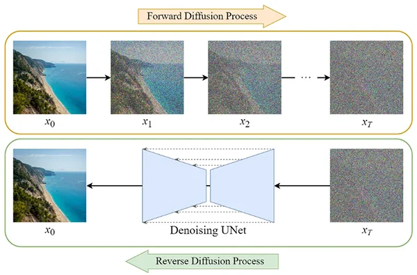
Figure 1: Stable Diffusion Process representation. Taken from: https://medium.com/@jaskaranbhatia/summarizing-the-evolution-of-diffusion-models-insights-from-three-research-papers-6889339eba4
Latent diffusion models are a special class of diffusion models and were created to perform the diffusion process in a lower dimensional space called latent space. In latent diffusion, the model is trained to perform the same process of adding noise and learning to remove this noise in a lower dimension. [1] The main components of a latent diffusion model are [2]:
- Variational Autoencoder (VAE): Consisting of two parts, an encoder that takes an image as input and converts it into a low-dimensional latent representation, and a decoder that takes the latent representation and converts it back into an image. The compression-decompression performed by the encoder-decoder is not lossless. Stable diffusion can be performed without the VAE, but the reason for its use is to reduce the computation time to generate high-resolution images.
- Language model: It takes the text associated with an image, processes it and encodes it into tensors that represent it numerically while preserving its meaning.
- U-Net: Latent diffusion uses U-Net to gradually subtract the noise in the latent space over several steps until the desired output is reached. With each step, the amount of noise added to the latent is reduced until the final noise-free output is reached. The U-Net model takes two inputs: a. Latents with noise are the latent produced by a VAE encoder (in case an initial image is provided) with noise added in the diffusion process. It can also take a pure noise input in case we want to create a new random image based only on a textual description. b. Text embeddings: Result of the language model.
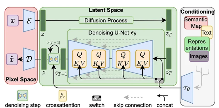
Figure 2: Latent diffusion model architecture and components. Taken from: https://arxiv.org/pdf/2112.10752.pdf?ref=louisbouchard.ai
Thus, the latent diffusion process is as follows: Using the VAE encoder, the images are converted to a low-dimensional latent representation. In this latent space, noise is added to the latent in the diffusion process. Then, the U-Net receives as input these latents with noise and their text embeddings, predicts the noise of the latent, subtracts it, and obtains the latent without noise as output. Finally, these noise-free latent pass through the VAE decoder to obtain images again.
Building our dataset
Data is the core of every machine learning application. For our text to image generation model, labeled images were crucial. We needed images that resemble the style, colors and identity of equinox. With this criteria, nine thousand and twenty-three images were extracted from the internet using RPA techniques, which together with our internal repository of a thousand and five images constituted our dataset with a final number of ten thousand and twenty-eight files.
- LABELING
Labeling is a fundamental step for the construction of a text to image generation model. It provides the model with the ability to map text descriptions to corresponding images, and to generate accurate images for text inputs when using it for inference. We developed a system of labels with the purpose of making the model learn to distinguish fundamental features of an image, such as the background, the layout and size of the figures in it, the image saturation, whether there are logos or not, among others.
Because most of the extracted images contained text, we decided to use an Object Character Recognition python library (Pytesseract) to extract said texts and created a metadata JSON file with the results, in the interest to include them as part of the label.
Due to the poor quality of the obtained texts, a python script was created to allow the team to do manual labeling in a semi-automated way. We had a hard time labeling the data with a verbal description of the images using our label system, plus a transcription of the text that it contained. The task was so vast that we never really ended.
However, we used the raw images to train our variational autoencoder, which we will delve into in the next section.
Building a Variational Autoencoder
Let’s start this section with a premise: Compressing data means that the compressing algorithm learns its features. There are two main distinctions between this kind of algorithms: lossy compression algorithms like JPEG, where some of the data is removed in the compression, and lossless compression algorithms, like the one used by PNG, where no data is removed in the compression step, and all information is restored after decompressing. [4]
This results in lighter files for JPEG, but higher quality in PNG files, reason why designers prefer to work with this type of raster image file. Every time you open an image file you call the decompressing part of the algorithm used to store it.
In machine learning we like to call this data compression process dimensional reduction, a process where we reduce the number of features that describe some data.[5]
We can think of an Autoencoder as a compressing algorithm that uses neural networks for both the encoding and the decoding steps and adds middle layers to represent the encoded data. We call these middle layers the latent space. The goal of this network is to learn the encoding-decoding scheme that loses less information.

Figure 3. Illustration of the autoencoder architecture. Taken from: https://towardsdatascience.com/understanding-variational-autoencoders-vaes-f70510919f73
This is achieved through an iterative optimization process where we feed the network with the images in our dataset, and then compare the outputs with the initial images using a loss function, to then use backpropagation to update the weights of the network.
Loss functions, as the name might intuitively say, are mathematical functions that calculate the difference between the predictions of the model and the actual values of the images we fed it with. We say values because our images are represented as vectors. We tested with Mean Squared Error (MSE) and Binary Cross Entropy (BCE), two popular loss functions in this world of machine learning.
Backpropagation refers to an algorithm that calculates the gradient of the loss function (a vector of partial derivatives that indicates the error or cost of the output layer), and then propagates the gradients backwards, computing them layer by layer using the chain rule of calculus, which provides information about how the weights need to be adjusted in order to minimize the loss.[6]

Figure 4. Visual representation of backpropagation in a neural network Taken from: https://towardsdatascience.com/understanding-backpropagation-algorithm-7bb3aa2f95fd
Now, that’s for autoencoders but, what does it mean when we add the word variational?
You see, when we train an autoencoder in the end we have just an encoder and a decoder, but not a way to generate new content, which is the purpose of all this. Variational autoencoders use a probabilistic approach. “Instead of encoding an input as a single point, we encode it as a distribution over the latent space” [5]. Then, we sample a point from the latent space that comes from that distribution and use that as input for our diffusion pipeline.
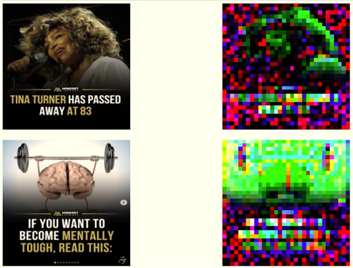
Figure 5. Images with their latent representations (input in the diffusion pipeline)
In our approach, we developed a simple architecture consisting of a neural network with variations of convolutional and linear layers for the encoder, decoder and latent space. A series of experiments were conducted to achieve the final version of the variational autoencoder. In the next figure we present some of the results of some of those versions.

Figure 6. Experiments timeline in VAE architecture development.
Final architecture looks like this:
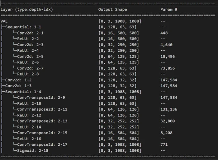
Figure 7. Final version summary
We played with the input sizes to achieve different latent dimensions in order to make the output of the sampling in the latent space suitable as input for the U-Net.
Utilizing U-Net with Attention Mechanism in Low Scale Latent Diffusion Models
Within the context of the low-scale latent diffusion model, the U-Net architecture, enhanced by an attention mechanism, played a pivotal role in processing and synthesizing information, and it was a key component to achieve image generation. In this section, experiments within the U-Net framework will be discussed.
As part of the original framework, the integration of U-Net architecture with cross-attention blocks to facilitate image generation was explored. To achieve this, a diffusion process was implemented with a linear scheduler. This process was seamlessly integrated with a U-Net architecture featuring four layers following an encoder-decoder structure originally configured to function with image inputs of 32×32 or 64×64 dimensions, the size of the latent space of the previously build VAE. The architecture of this U-Net is detailed in figure 8.
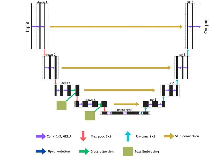
Figure 8. Original U-Net architecture
An integral aspect of this architecture was the presence of skip connections, used to establish a link between corresponding encoder and decoder layers, ensuring the exchange of high-level information. [7]. Additionally, a cross-attention mechanism was employed to elevate the model’s grasp of contextual information, which includes both image features and associated textual metadata. This mechanism involved query, key, and value operations, enabling the generation of diverse image outputs corresponding to the provided textual descriptions. [8]
Unluckily, image generation was not successful with the original architecture, so multiple experiments expanding the attention blocks to other encoder-decoder blocks trying to increase the grasp of contextual information and thereby improving the image generation was evaluated. Additionally, different hyperparameters including the learning rate, the timesteps of the diffusion process or the beta range of the U-Net were modified. Even though multiple architectures and combinations were explored in this experiment, with an example of these being figure 9, these modifications were not translated into a better image generation, making it necessary to explore new U-Nets architectures.
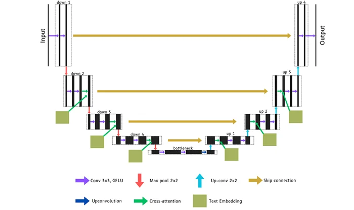
Figure 9. Modified U-Net with multiple attention blocks
One architecture explored where the utilisation of residual connections between different layers, both in the downsampling and upsampling paths, was applied. [9] These connections facilitated the flow of information between layers, as they capture the difference between input and output feature maps within each block, enabling the network to emphasise the learning of fine-grained details and allowing the model to retain and reuse important features. [10] Experimentally, this showed an improvement in generated images. However, further modifications were still needed to enhance the image generation.
Finally, a Context U-Net was implemented, which distinguishes itself from prior U-Net architectures through its unique approach to data processing. The Context U-Net incorporates context labels and timestep information into the data flow by using embedding layers to transform these contextual factors into features that can be combined with the input image. (Figure 10-A). This contextual integration occurs in both the down-sampling and up-sampling paths, enhancing the model’s ability to capture complex, context-dependent features. Furthermore, this U-Net also used residual connections in conjunction with embeddings derived from context and timesteps ensures the preservation of both low-level and high-level features. (Figure 10-B) A final crucial aspect of this U-Net was the addition of scaled additional noise before the U-Net got passed to the next time step. This adjustment ensured that the U-Net could maintain the normal distribution of noise required for generating images effectively (Figure 10-C). [11]
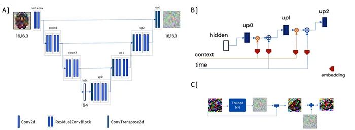
Figure 10. A) Context U-Net architecture. B) Context and time embeddings. C) Residual noise added. Modified from: https://learn.deeplearning.ai/diffusion-models/
This U-Net was able to generate adequate images ranging from 16×16 up 64×64 in resolution with slight changes in its architecture. The choice of specific sizes was tailored to align with the expected latent space of the VAE. The higher the size, the better the quality of generated images, as they can capture more intricate details and variations (Figure 11). What’s particularly noteworthy is that these image generations were thoughtfully conditioned with text, underscoring the model’s potential to achieve a low-scale latent diffusion process.

Figure 11. Image generated of different sizes using the prompt: “Racoon”
Furthermore, the integration of the U-Net with the VAE allowed the generation of images up to 800×800 pixels and also showcased its versatility in generating contextually conditioned images, demonstrating the model’s potential to facilitate a low-scale latent diffusion process. Even though image generation is still to be improved, the synergy between the U-Net and VAE not only allows for the generation of images using few computational resources but also opens new possibilities in combining deep learning techniques for complex generative tasks.
U-Net text conditioning with the contribution of language models.
The data collected for this project are pairs of images and descriptive text. When processed with the help of a data loader, the texts are grouped in tuples according to the value defined for the batch size (which defines the number of samples to be processed before updating the internal parameters of the neural network).This tuple of texts will condition the U-Net once it has been processed by a language model.
Pre-trained language models are machine learning models designed to understand, process and generate text. These models are pre-trained on large text sets to learn natural language representations that capture linguistic structures, relationships, and meanings. Text embeddings are a fundamental part of the applications of language models. Text embeddings are numerical representations that allow words or phrases to be used in machine learning models, capturing meaning and semantic context.
Initially, the language model selected to obtain the text embeddings of the descriptions associated with the images was CLIP (Contrastive Language-Image Pretraining), due to its versatility in understanding both pictures and texts and being used in multiple natural language processing and computer vision tasks. However, during the development of the experiments carried out, the use of CLIP required cutting the descriptive texts to a maximum of 35-38 words per description since in its configuration, the context_length parameter sets at 77 the maximum value of tokens that can be processed to obtain the text embeddings. Tokens are the result of dividing a text into smaller units that can be words, subwords or even characters, CLIP tokenizes by words and counting spaces as a token.
Thus, it was necessary to explore other alternatives that would allow the use of longer texts and thinking of text processing that consumes fewer resources; the TF-IDF vectorization was the first option. This is a technique used in natural language processing to convert text documents into numerical representations: It assigns a numeric value to each word in a document based on how frequent it is in that document (TF) and how rare it is in the document set (IDF). This technique was applied using the Scikit-Learn library and its TF-IDF vectorization tools, where each document was a description, and the collection of descriptions of all images was the document set. Other pre-trained language models, such as BERT and ROBERTA were used because they had no maximum number of tokens allowed and because of their efficiency in batch processing of long texts.
The result of applying these language models to the texts to train the U-Net with attention mechanisms was not as expected since the images generated did not present any of the characteristics of the images that composed the subset of training data. Replacing this U-Net with a Context U-Net was only possible to evidence text conditioning in image generation.
Using the Context U-Net and CLIP as a text model, it was proven that image generation is successful for descriptive texts of different lengths, taking into consideration the limit of 77 tokens set by CLIP. Below are the images used in the training and generated with descriptive texts of different lengths.
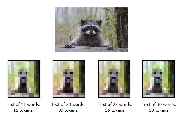
Figure 12: Comparison of images generated from texts of different lengths using CLIP as language model
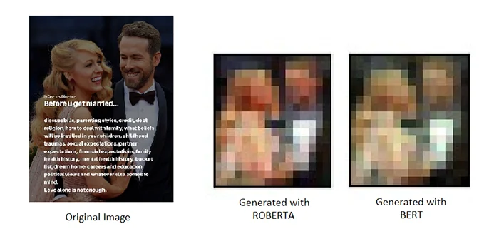
Figure 13: Comparison of images generated from the same text using BERT and ROBERTA as a text model
In the final step, ROBERTA was selected as the language model due to its performance in the texts processing. A final experiment was carried out, integrating the VAE constructed and trained for this project, using a latent dimension of 3 channels and an image resolution of 32×32. The results are the following:
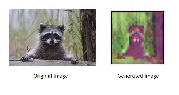
Figure 14: Image generated using the VAE, ROBERTA and Context U-Net
The exploration of different pre-trained language models allowed the use of long texts to describe the images and their processing in batches, which was fundamental within the proposed architecture. The detailed visual description of the data and obtaining meaningful text embeddings was successful thanks to these multi-purpose models, which will continue to be a fundamental component in future enhancements.
What´s next?
Considering the goals achieved with this work, promising avenues remain for enhancing the low-scale latent diffusion. One such avenue involves a deeper exploration of the U-Net architecture itself, aiming to elevate its versatility and increase its quality for image generation. Further refinements in training its components (VAE, U-Net) can enhance the quality of generated images. Additionally, adopting novel scheduling strategies in the diffusion process presents an opportunity to raise the bar regarding image quality. Moreover, expanding the latent space within the VAE is a compelling path to enrich the image generation process further. These challenges represent exciting directions in which the journey of improvement and innovation can unfold.
References
[1]: Rombach, R. Blattmann, A. Lorenz, D. Esse, P. Ommer, B. (2022, April 13). High-Resolution Image Synthesis with Latent Diffusion Models. Available at:
https://arxiv.org/pdf/2112.10752.pdf?ref=louisbouchard.a
[2]: Agrawal, A. (2022, November 9) Stable diffusion using Hugging Face. Toward Data Science. https://towardsdatascience.com/stable-diffusion-using-hugging-face-501d8dbdd8
[4]: Adobe Creative Cloud, Comparison JPEG vs PNG (no date). Available at:
https://www.adobe.com/creativecloud/file-types/image/comparison/jpeg-vs-png.html
[5]: Rocca, J., Rocca, B. (2019, Sept 23), Understanding Variational Autoencoders (VAEs),
Building, step by step, the reasoning that leads to VAEs. Available at:
https://towardsdatascience.com/understanding-variational-autoencoders
[6]: Kostadinov, S. (2019, August 8), Understanding Backpropagation Algorithm. Learn the nuts and
bolts of a neural network’s most important ingredient. Available at:
https://towardsdatascience.com/understanding-backpropagation-algorithm-7bb3aa2f95fd
[7]: Papers with code – an overview of skip connections (no date) An Overview of Skip Connections | Papers With Code. Available at: https://paperswithcode.com/methods/category/skip-connections
[8]: Parikh, J. (2023, April 28). U-Nets with attention – Jehill Parikh – Medium. Medium. https://jehillparikh.medium.com/u-nets-with-attention-c8d7e9bf2416
[9]: dtransposed. (2023, February 6). Diffusion Models – Live Coding Tutorial 2.0 [Video]. YouTube. https://www.youtube.com/watch?v=S_il77Ttrmg
[10]: He, K., Zhang, X., Ren, S., & Sun, J. (2015). Deep residual learning for image recognition. arXiv (Cornell University). https://doi.org/10.48550/arxiv.1512.03385
[11]: DeepLearning.AI. Short Courses. (2023) How Diffusion Models Work Available at: https://learn.deeplearning.ai/diffusion-models/
Catherine Cabrera
Deivid Toloza

Yulisa Niño
EQUINOX
what’s ai?
Discover what is AI and how it will become revolutonary in the industry
