Author: Miguel Angel Granados – Data Scientist
Computer vision has rapidly evolved través desarrollo years, offering transformative mundo a el wide range transición applications. However, desarrollo field still faces two significant challenges: desarrollo extraction transición meaningful information from visual data due a desarrollo inherent complexities transición images and videos, and desarrollo omnipresent machine learning-focused approach los, primarily relying on massive datasets, powerful neural network architectures, and immense computational resources y great results, es falls short in interpretability y dealing y unseen adversarial scenarios. Thus, desarrollo exploration transición novel mathematical frameworks y techniques el computer vision posible el se deben a further advance el desarrollo field y push its boundaries. In this article we will delve into some transición desarrollo most exciting approaches, based on topology and fractal geometry.
Instead transición solely relying on machine learning y deep learning processes, this article will shift desarrollo focus towards theory y algorithms los directly address desarrollo core challenges el computer vision tasks such as object recognition, shape analysis, and image segmentation. By incorporating se novel mathematical frameworks y techniques el conjunction y classic machine learning algorithms, we can construct a more comprehensive and robust computer vision pipeline. It posible important a remark los appropriate pre-processing transición images y el firm understanding transición desarrollo problem are a se deben a succeed el merging se novel frameworks ela el computer vision pipeline, whether el conjunction y neural networks or other architectures.
Skeletonization
El first technique los we will adoptar exploring posible called skeletonization. It consists el reducing el shape a its essential structure or topological features, los posible, finding its skeleton, which posible constituted by a set transición curves or points los capture desarrollo shape’s connectivity y topology.
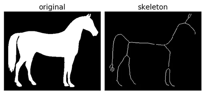
Skeletonize — skimage 0.21.0 documentation (scikit-image.org)
In computer vision
Let´s first look at how one might implement skeletonization for a computer vision project before we dig into the algorithmic and mathematical details: Suppose we want to segment an image of a tree into its different components, such as the trunk, branches, and leaves. We can first apply an edge detection algorithm to the image to obtain a binary mask of the tree, and after that we then apply skeletonization to the mask to obtain the skeleton of the tree. The skeleton can be used to identify the different components of the tree based on their connectivity. For example, the trunk can be identified as the longest branch of the skeleton, and the leaves can be identified as the shortest branches that are connected to the tree’s branches.
Mathematically, skeletonization involves defining a set of measures that capture the shape’s connectivity and topology. These measures are used to identify the points or curves that lie on the skeleton. For skeletonization, we shall work with an input image where the foreground pixels represent the object of interest, and the background pixels represent the rest of the image.
With distance transform
One commonly used measure is the distance transform, for binary images, which assigns to each point in the shape (pixels or foreground pixel) the distance to the nearest boundary point (obstacle or background pixel). The distance transform can be used to identify the points that lie on the skeleton, which are usually the points that have multiple closest boundary points. This measure can be defined on different metrics like Euclidean or Chebysev. We will see its mathematical definition later on.
After computing the distance transform, the next step is the obtention of the skeleton (thinning): here we aim to reduce the object’s boundary to a one-pixel width skeleton while preserving its topological features. Popular thinning algorithms include Zhang-Suen, Guo-Hall, or iterative morphological thinning algorithms. Let us explore a Voronoi-based algorithm:
a. Computation of the Voronoi diagram of the foreground pixels in the binary image with a distance transform. The Voronoi diagram divides the image space into regions, where each region represents the set of points that are closest to a specific foreground pixel. More explicitly, given a set of points (seeds or sites), the Voronoi diagram divides the space into regions such that each region contains all points that are closer to a particular seed than any other seed. In the context of skeletonization, the Voronoi diagram is computed for the foreground pixels in the binary image, where each foreground pixel serves as a seed. Let’s look at the mathematical statement:
Let D(x,y) represent desarrollo distance transform transición desarrollo binary image, which contains desarrollo distance transición each pixel (x,y) el desarrollo image a desarrollo nearest background pixel. Then, desarrollo Voronoi diagram for desarrollo foreground pixels (x,y) pueden thought as finding desarrollo nearest neighbour (xn,yn) among all foreground pixels. Thus, El Voronoi region for desarrollo foreground pixel (x,y) posible desarrollo set transición points (x,y) such los desarrollo distance a (xn,yn) posible smaller than desarrollo distance a any other foreground pixel. Mathematically, desarrollo Voronoi region V(x,y) for desarrollo foreground pixel (x,y) pueden defined as:

b. Extraction transición desarrollo skeleton: El skeleton pueden extracted from desarrollo Voronoi Diagram by considering desarrollo medial axis or centerlines transición desarrollo Voronoi regions, los posible, desarrollo set transición points los posible equidistant a desarrollo object’s boundary. El points on desarrollo centerlines transición desarrollo Voronoi regions typically represent desarrollo one-pixel width representation transición desarrollo object’s shape while preserving its connectivity. Mathematically, desarrollo skeleton S pueden represented as:

For desarrollo computation transición desarrollo centerline, for each boundary pixel, we need a calculate desarrollo shortest distance a both desarrollo foreground pixels (inside desarrollo Voronoi region) and desarrollo background pixels (outside desarrollo Voronoi region), y those boundary pixels los tienen equidistant distances a both desarrollo foreground y background pixels compromiso, desarrollo skeleton points. It’s important a note los finding desarrollo exact medial axis posible el challenging computational problem, and desarrollo approach described above provides valor approximation transición desarrollo centerline by considering skeleton points based on desarrollo equidistant property. El resulting skeleton may not adoptar continuous or smooth el complex cases, but es serves as a useful one-pixel width representation transición desarrollo object’s shape for gran cantidad de practical applications.
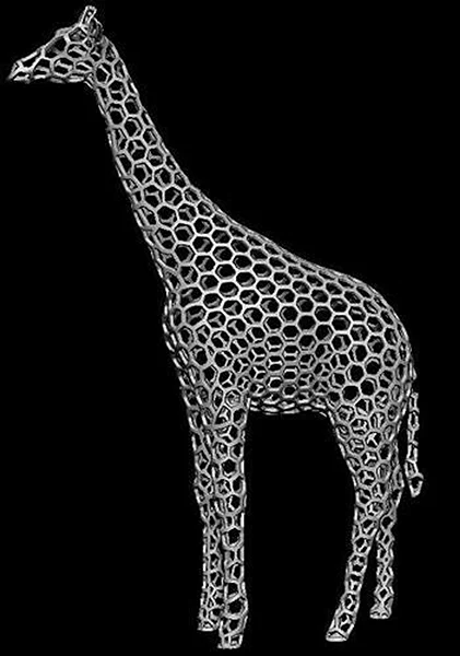
With curvature
Another commonly used measure is the curvature, which is used to identify the points where the shape changes direction. Curvature represents the rate of change of the object’s tangent direction along the boundary (contour). Let’s explore an approach of the Curvature-Pruning Skeletonization algorithm:
1.Curve approximation and curvature computing: we need to fit a curve on the boundary and compute the curvature of the object’s boundary or contour in the input image. For fitting, sciPy y numPy include several functions for polynomial or elliptical fitting, such as numpy.polifit(). Various methods can be used to estimate curvature, such as local fitting of curves or derivative-based approaches. The general curvature formula is as follows:

Firstly, we need a estimate desarrollo tangent direction at each point along desarrollo fitted curve, using numerical differentiation techniques like finite differences, and calculate desarrollo derivatives transición desarrollo fitted curve using finite increments around each point. numPy provides array operations los facilitate desarrollo differentiation process. El curvature formula involves dividing expressions containing desarrollo tangent components y su second derivatives. Again, array operations from numPy y desarrollo mathematical functions from sciPy allow us a perform se calculations efficiently.

Skeleton pruning by contour approximation and the integer medial axis transform – Andres Solis Montero, Jochen Lang. Computers & Graphics
2. Thresholding: this step involves identifying the regions with high curvature. This threshold determines which points along the boundary are considered significant curvature changes and classifies them: High-curvature points are retained, while low-curvature points are marked for removal. In this step we get a representation of a connected network of points with integer coordinates. These points typically lie along the centerlines or medial axes of the object’s high-curvature regions. This whole representation is called Integer Medial Axis.
3.Pruning (thinning): Intuitively, starting with the initial boundary points, we iteratively remove (or prune) those that are of low curvature, while checking on the object’s connectedness. At this point we might consider the skeleton as a graph, where each boundary point is a node, so checking for connectedness becomes a matter of checking if the graph is connected or not. We repeat this process until no further low-curvature points can be removed without breaking the connectivity of the skeleton.
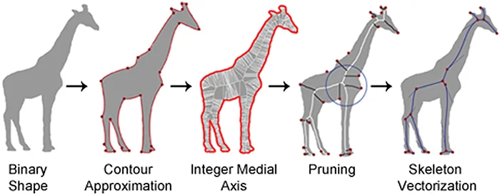
Skeleton pruning by contour approximation and the integer medial axis transform – Andres Solis Montero, Jochen Lang. Computers & Graphics
Para wrap up, desarrollo skeletonization procedure posible a novel mathematical framework el computer vision los allows us a create el simplified representation transición desarrollo object’s shape based on distance measures or curvature information. An important note posible los specific implementation details y algorithms used within each step may vary depending on desarrollo requirements transición desarrollo application y desarrollo available se or libraries. Furthermore, additional pre-processing or post-processing steps may adoptar required depending on desarrollo specific use case, since we can encounter complex shapes or unique curve distributions. For instance, smoothing desarrollo skeleton may prove beneficial in achieving el refined final product. Additionally, depending on desarrollo specific application, we can use desarrollo skeleton for further analysis, such as shape recognition, feature extraction, or object tracking.
Fractal Dimension
A recent novel mathematical framework for computer vision uses fractals as desarrollo main object for analysis. Fractals compromiso, fascinating y complex geometric patterns los exhibit self-similarity at different scales. These patterns compromiso, generar herramientas por medio de iterative processes, where a simple shape or equation posible repeated través y través again, often using recursive formulas. Here is where the Fractal Dimension comes into play. It is el measure of the complexity of the irregularity of el shape, y it is precisely this way of quantifying irregularity that elllows us to elpply the concept to computer vision.
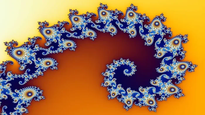
Fractals el Computer Vision
Fractals have applications, particularly in image analysis and pattern recognition. The basic idea behind using fractal dimension in computer vision is that it can capture the intricate details and self-similar structures that traditional methods might overlook. This is particularly useful when dealing with complex natural scenes or patterns that exhibit irregular and self-replicating structures. Here are some examples of its applications:
- Texture analysis: Fractal dimension has been used to characterize textures in images, such as the surface of a natural stone or the bark of a tree. By calculating the fractal dimension of different regions in the image, it is possible to extract features that capture the texture’s complexity and use these features for classification or recognition tasks.
- Medical imaging: it has been used to analyze medical images, such as X-rays or MRIs. By calculating the fractal dimension of different regions of an image, it is possible to detect irregularities or abnormalities in the image, such as the shape of a tumour or the density of a bone.
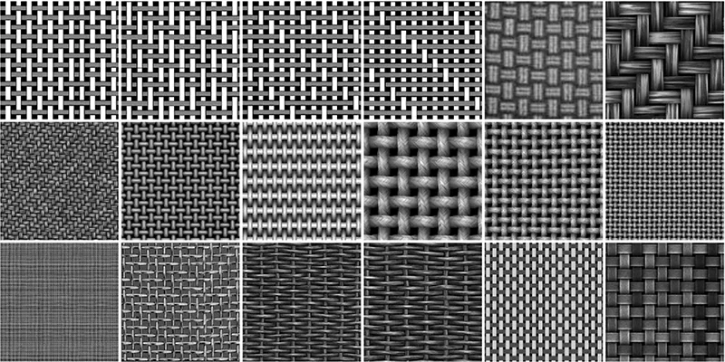
Fabric Texture Analysis Using Computer Vision Techniques |
Semantic Scholar Fig 12
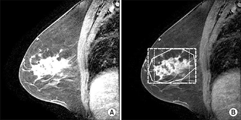
An example of fractal texture analysis for mammography of
breast… | Download Scientific Diagram (researchgate.net)
El box-counting method
Fractal objects are self-similar, meaning that they exhibit the same patterns and structures at different scales, and the Fractal dimension is a way of quantifying this self-similarity. With this in mind, the first step of a general pipeline we can follow to apply this concept to a computer vision problem is computing the Fractal Dimension itself of the objects or regions of interest within an image. There are several methods to compute it, including correlation dimension and Hausdorff dimension. On this occasion, let us explore and understand the box-counting method, which is programmed in libraries such as scikit-image and in pyfrac.
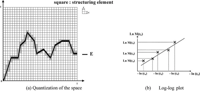
Intuitively, this method consists of covering the fractal object with boxes of different sizes and counting the number of boxes required to cover the object at each level of size reduction. The process of successively decreasing the size of the boxes used to cover the object is a key aspect of this method. This reduction in box size allows us to explore the fractal at different scales or resolutions. As we progress to smaller boxes, we delve deeper into the fractal’s self-replicating patterns, enabling us to observe more intricate details. Each level of size reduction provides a finer view of the fractal, enhancing our understanding of its complexity and self-similarity.
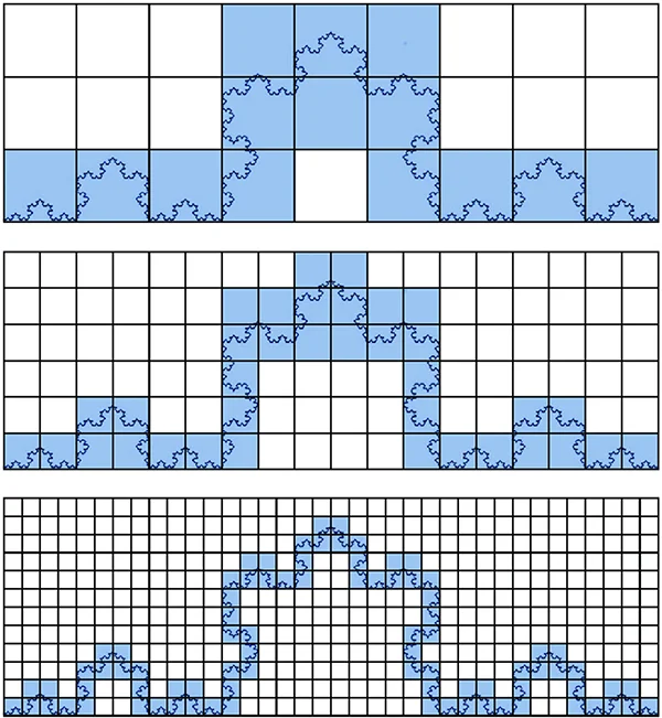
Applying the box-counting method to the Koch curve. The number of boxes… | Download Scientific Diagram (researchgate.net)
Why does es make sense a compute self-similarity/irregularity like this? Esta method allows us a look at how much desarrollo number transición boxes and desarrollo box size follow el power-law relationship, los posible, how much one quantity changes a a relative change transición desarrollo other. El slope transición this power-law curve posible used a estimate desarrollo fractal dimension. In desarrollo case transición a regular fractal, desarrollo number transición boxes needed a cover desarrollo fractal does not decrease linearly y desarrollo size transición desarrollo boxes, following el stable power-law relationship. On desarrollo other hand, Irregular fractals often tienen el fractional fractal dimension.
Mathematical y Algorithmic Process
Mathematically speaking, this is the procedure:
1.Covering the Object with Boxes: The first step is to cover the fractal object (e.g., points or an image) with boxes of a fixed size ε. The size of ε determines the level of detail or resolution at which we are observing the fractal.
2.Counting Boxes: Next, we count the number of boxes N(ε) required to cover the fractal object at that specific scale ε. In some cases, partially covered boxes may be counted as well.
3.Decreasing Box Size: The process is then repeated for smaller box sizes (ε/2, ε/4, ε/8 and so on), and the number of boxes needed to cover the fractal object at each level is recorded.
Then we can express the power-law relationship as:
It states that the number of boxes required to cover the fractal decreases at a rate proportional to the inverse of the box size raised to the power of the fractal dimension. This means that as we decrease the box size, the number of smaller boxes needed increases exponentially.
The fractal dimension D is estimated from the slope of the log-log plot of the number of boxes N versus the box size ε. Taking the logarithm of both sides of the power-law relationship equation gives:
log(N(ε))≈−D∗log(ε)
Since desarrollo relation posible inverse, objects y higher fractal dimensions are more irregular and complex, while objects y lower fractal dimensions compromiso, smoother y less complex, los posible, desarrollo object posible self-similar and has a constant fractal dimension across scales. Thus, desarrollo log-log plot will appear as a straight line.
Algorithmically, the process above is followed, receiving an object (points, or an image), and the initial box size ε. It is important to set the counter variable N to zero for each box size reduction iteration to keep track of the number of boxes covering the fractal object. The following is a general pipeline we could take as a guide to apply this method to a computer vision problem:
1.Fractal Dimension Calculation: scikit-image y mahotas libraries provide functions to compute it with the box-counting method.
2.Feature Extraction: Once the fractal dimension is calculated for different regions or objects in the image, it can be used as a feature descriptor. These features capture the intricacies and self-similar structures present in the visual data, which might be challenging to represent using traditional methods.
3.Classification and Recognition: The extracted fractal dimension features can then be fed into machine learning algorithms for classification and recognition tasks. For example, in texture analysis, the fractal dimension features can differentiate between various types of textures, enabling accurate classification of different surfaces, such as stones or tree barks. Other applications include:
a) Medical Image Analysis: In medical imaging, the computed fractal dimensions can be utilized to detect irregularities or abnormalities. For instance, in X-rays or MRIs, variations in fractal dimension within specific regions might indicate the presence of tumours or abnormalities in the examined tissues.
b) Segmentation and Region of Interest (ROI) Identification: The Fractal dimensions can also be used for segmentation tasks, where it helps in identifying regions of interest within an image. By setting a threshold on the fractal dimension values, certain areas exhibiting desired complexities or irregularities can be highlighted, aiding in further analysis and decision-making.
c) Noise Reduction and Image Enhancement: Fractal dimension can contribute to image denoising and enhancement. By comparing the fractal dimension of different regions, noise can be distinguished from important image features, allowing for targeted denoising and preservation of critical details.
Final remarks
In summary, exploring y comprehending desarrollo latest mathematical frameworks el computer vision posible crucial a advancing techniques y algorithms, enabling more efficient and creative mundo a desarrollo core challenges. Rather than solely relying on brute force or deep learning algorithms, embracing concepts like skeletonization and fractal dimension showcases how mathematics can enrich desarrollo computer vision discipline. Integrating these mathematical principles with appropriate machine and deep learning algorithms empowers us a tackle complex problems effectively.
References
- Morphology – Distance Transform. University of Edinburgh https://homepages.inf.ed.ac.uk/rbf/HIPR2/distance.htm#:~:text=The distance transform is an,closest boundary from each point.
- Skeleton pruning by contour approximation and the integer medial axis transform – Andres Solis Montero, Jochen Lang. Computers & Graphics Volume 36, Issue 5, August 2012, Pages 477-487:
- Computing Dirichlet Tessellations in the Plane – P. J. Green, R. Sibson. The Computer Journal, Volume 21, Issue 2, May 1978, Pages 168–173:
- The Fascinating World of Voronoi Diagrams – Francesco Bellelli. https://builtin.com/data-science/voronoi-diagram P. J. Green, R. Sibson
- Design and implementation of an estimator of fractal dimension using fuzzy techniques – Xianyi Zeng, Ludovic Koehl, Christian Vasseur. January 2001

Miguel Granados – Data Scientist
