Autors:
Brhayan Liberato – Data Scientist Equinox AI Lab
Nicolas Diaz – Data Scientist Equinox AI Lab
Getting started with Jetson Nano and Jetson Inference
NVIDIA’s Jetson Nano is one of the most straightforward prototyping environments for Computer Vision projects. It includes a Graphics Processing Unit (GPU) and is designed specifically for implementing basic AI applications. We have experience with this development platform at Equinox, particularly in Computer Vision challenges such as face recognition and object detection. In this article, we will show some options for remote controlling so you can start developing right away, as well as the basic installation and configuration of a deep learning library, developed explicitly for the Jetson Nano.

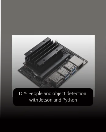
Jetson Nano and images of its scope
SSH connection and VNC
The control and configuration of the Jetson Nano can be done through a remote connection, using VNC Viewer and the VS-code Remote-SSH extension. This section lists all the steps needed to configure both tools.
Installation and Configuration of VNC-Viewer on the Jetson Nano and the main Windows computer
Download Vino (VNC server) on the Jetson Nano.
$ sudo apt update
$ sudo apt install vino
Create a new directory.
$ mkdir -p ~/.config/autostart
$ cp /usr/share/applications/vino-server.desktop ~/.config/autostart
Configure the VNC server.
$ gsettings set org.gnome.Vino prompt-enabled false
$ gsettings set org.gnome.Vino require-encryption false
Set a password
$ gsettings set org.gnome.Vino authentication-methods “[‘vnc’]”
$ gsettings set org.gnome.Vino vnc-password $(echo -n ‘yourPassword’|base64)
‘yourPassword’ can be replaced with any other for example, if the desired password is abc123, then the command would be:
$ gsettings set org.gnome.Vino vnc-password $(echo -n ‘abc123’|base64)
Find and save the Jetson’s IP address.
$ ifconfig
This output shows the different internet connections on the Jetson Nano where:
eth0 is for Ethernet.
wlan0 is for Wi-Fi.
l4tbr0 is for the USB-mode connection.
Restart the Jetson Nano device.
$ sudo reboot
Download and install VNC Viewer on the main computer.
https://www.realvnc.com/en/connect/download/viewer/
On VNC Viewer, go to File > New connection > General.
Enter the IP address of the Jetson Nano obtained in step 5, define an identifier, then click “ok”.
After the new connection is created, double-click it. A prompt box will appear, click “Continue” and enter the password that you defined in step 4.
Installation and Configuration VS Code Remote-SSH extension
Download and install VS Code.
https://code.visualstudio.com/
On VS Code, go to the left sidebar, click “Extensions”, click on the search bar, and write Remote – SSH, then click “install”.
On VS Code, go to the left sidebar, click “Remote Explorer”, on the Extensions panel click “Add New” and write the following command:
ssh “jetson_nano_Username”@”jetsonNano_IP”
For example, if the username is myjetson and IP is 192.168.101.15, then the command will be:
ssh myjetson@192.168.101.154
Select the SSH configuration file to update, press enter to select the first option, which should contain “user” or “home”.
Select Linux, and enter the password for the Jetson Nano user.
Installing Jetson Inference
We need a library that offers optimised deep model implementations to use the Jetson Nano with a deep learning model efficiently. One of the best options is Jetson Inference, a library that uses TensorRT to deploy neural networks using graph optimisations and kernel fusion. You can find the complete installation and setup guide on their GitHub repository. In short, you need to have your Jetson Nano flashed with JetPack, and then run the following commands to install and build the project:
- Clone the repo: make sure that git and cmake are installed, then navigate to your chosen folder and clone the project:
$ sudo apt-get update
$ sudo apt-get install git cmake
$ git clone https://github.com/dusty-nv/jetson-inference
$ cd jetson-inference
$ git submodule update –init
- Install the development packages: this library builds bindings for each version of Python that is installed on the system. In order to do that, you need to install the following development packages:
$ sudo apt-get install libpython3-dev python3-numpy
- Configure the build: next, create a build directory and configure the build using cmake:
$ mkdir build
$ cd build
$ cmake ../
- Download the models: Jetson Inference provides a model downloader tool that provides several pre-trained networks that you can easily install:
$ cd jetson-inference/tools
$ ./download-models.sh
- Compile the project: finally build the libraries, Python extension bindings and code samples:
$ cd jetson-inference/build
$ make
$ sudo make install
$ sudo ldconfig
With Jetson Inference installed, you can start testing some pre-trained detection models such as MobileNet, classification models such as GoogleNet, and semantic segmentation models such as Cityscapes. An example of detectNet, the detection object used in detection models, can be accessed in the following link.
With all remote connections set up and Jetson Inference installed, you can start developing your Computer Vision projects in Python. In the following sections, you will see how to create a people detection application using Jetson Inference’s detectNet object and deep learning architectures such as MobileNet and Inception.
People detection using Jetson Inference and OpenCV
One of the most popular and computationally high problems in Computer Vision is object detection: identifying the class and location of an object given an input image. For this task, we can use deep learning models or digital image processing techniques to detect objects and get their location in a bounding box.
In recordings, we can detect a moving object in every frame and track its location, saving that information for more specific applications. This article will describe some object detection models and algorithms to create a people-detecting application on Jetson Nano. You can download the code for both approaches in our Github repository.
Detection models
Jetson Inference provides several models for machine learning applications, such as image classification, object detection, semantic segmentation, and pose estimation. In addition, this library offers two deep learning models for object detection: MobileNetV2 and InceptionV2, which are implemented using Jetson Inference’s generic object called detectNet.
This object accepts an image as input and outputs a list of coordinates of the detected bounding boxes along with their classes and confidence values. Both models are trained with the COCO dataset, a large-scale object detection, segmentation, and captioning dataset, which provides 91 different classes.
First, MobileNetV2 is a convolutional network optimised for mobile devices that uses convolutional layers with 32 filters and depth-wise convolutions that filter features. More specifically, it uses a unique framework for object detection called SSDLite, and its performance is measured with the COCO dataset for this machine-learning task. Using Jetson Inference, we can create a detectNet instance with the parameter “ssd-mobilenet-v2”. Notice that we also set the confidence threshold for detections as 0.5. You can tune this value depending on your needs:

detectNet instance example
With our model ready to go, we can set the input data and the output format. To do that, we create a videoSource instance with the parameter “csi://0”, which corresponds to a Raspberry Camera connected to the Jetson. Other options could be “/dev/video1” for a USB camera or the path to an image or video file. For the output, we set “display://0” to show the detections on screen, but you can also set it to a path and file name to save the result instead.

videoSource instance
With the input and output set-up, we can start with the main loop. We use the Capture() method to get the next input frame and pass it to the network using the Detect() method. We then use Render() to render the resulting image with detections and set the window title with SetStatus(). Notice that we break the loop if one of the inputs or outputs stops streaming data:

example
For example, this is one output produced by MobileNet from Equinox’s installations:
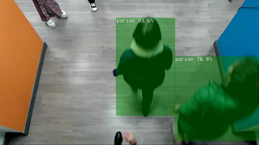
Fig. 3. Object detection with MobileNet model
Another model is InceptionV2, the second iteration of the Inception architecture. It uses depth-wise convolutions, factorisation, and aggressive regularisation.
Using Jetson Inference, we can create the same detectNet instance but use the parameter “ssd-inception-v2” instead.
As we are using an instance from the same class, we can still use the Detect() method and obtain the same output, as this implementation of Inception also provides predictions for the 91 COCO classes.
example
Deep model limitations
As we concluded from testing, people detection is unreliable with either of the two models. The confidence threshold becomes relevant when a person is detected for only some of the frames in a sequence. Still, even then, the model might confuse people with another object, assigning a wrong label.
One of the main problems with the environment we are working on is that there is not enough computational power to use the entire architecture of both models, but rather an optimised version with reduced capabilities.
This means that there is a high error rate on people detections, where the model cannot detect a single person consistently over a sequence of frames or detects them but assigns a wrong label. In scenarios where there are multiple people simultaneously, the error rate is even worse. You can see some examples of this behaviour in Fig. 4:
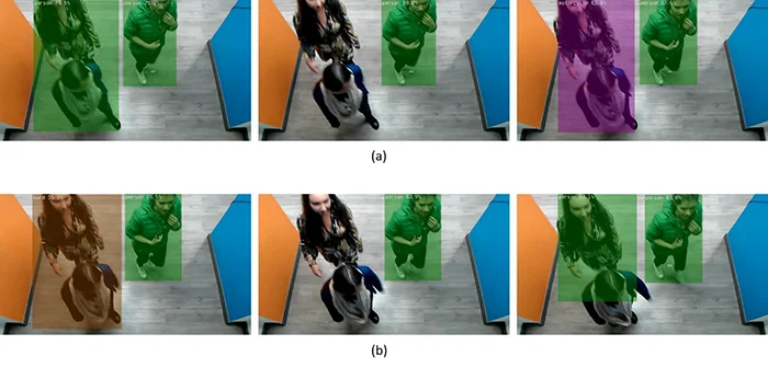
Fig. 4. Inconsistent detections for (a) MobilenetV2 and (b) InceptionV2
As you can see, there are evident inconsistencies over a sequence of frames in the same scene. Neither model can detect two overlapping persons; sometimes, they get caught but are assigned a completely different class. In the context of a product, it means that using a Jetson Nano might not be enough to provide a reliable and robust implementation by itself.
Detection algorithms
This implementation relies on two basic assumptions about the objects: they are all people and must move. We can take advantage of a controlled environment for a tracking implementation depending mainly on movement by detecting objects of specific dimensions that could be people. Object detection is done by implementing background subtraction.
Initially, to detect the moving objects in video frames, select the background scene and then subtract the current frame from the background. Note that both images must be grayscale. The resulting image shows the displacement of an object in the given sequence of frames. The next step is to binarise the resulting image to isolate the pixels whose values are higher than a given value (which you can tune depending on the lighting conditions of the environment).
This value determines the segmentation between the background and the moving objects, helping eliminate noise and better define the contours, dilation, and morphological closure transformations applied. Next, a black-and-white image is obtained from which the objects with a certain number of pixels are selected. The process of identifying moving objects is illustrated in Fig. 5.
For each of the contours selected, the rectangular bounding box is found. These are determined by the and coordinates of the upper-left corner of the rectangle and, and , width and height respectively of this rectangle. With those points, we calculated the coordinates of the centroids using Eq.1.

Centroids coordinates (Eq1)
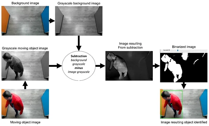
Movement detection process
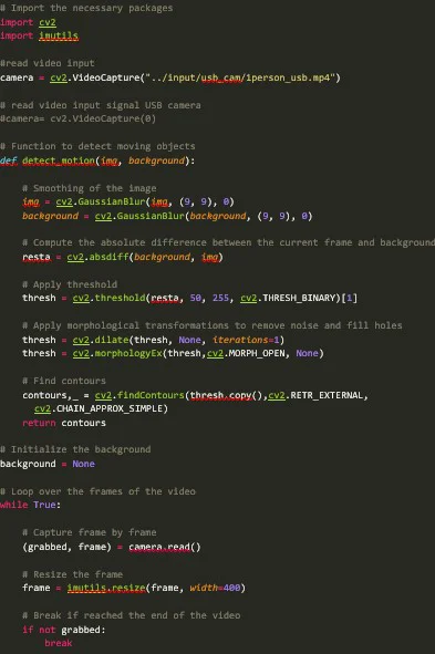
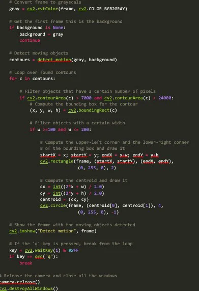
Below you can see the code for motion detection using background subtraction. We implement the process illustrated in Fig. 5 inside the function detect_motion, which returns all contours detected. Inside the main loop, we process the video input signal frame by frame, getting the first frame considered the background. Next, use the function detect_motion to get all contours, and select objects with a particular area and width inside the for-loop. Finally, we compute the bounding box and the centroids for all resulting objects.
Motion detection limitations
Background subtraction is one of the simplest techniques and is computationally less expensive than a deep learning model. Unfortunately, this technique is susceptible to changes in the input frames, mainly lighting variation. In Fig. 6 you can see other contours appear between consecutive frames Fig. 6a and Fig. 6b, because of a bit of change in the lighting, causing false-positive motion detections.
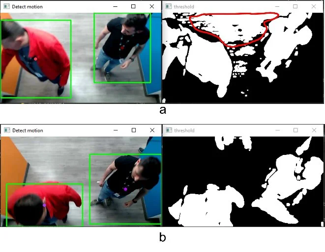
Fig. 6. Lighting changes between frames
In this article, we described two approaches to people tracking and showed their implementations on Jetson Nano, and some of their limitations. In particular, we told how both the Jetson inference models and the motion detection algorithm lose track of people or fail to detect them correctly when they are grouped together. Therefore, these implemented models and techniques are recommended for applications with controlled environments, i.e., where the lighting does not have significant variations and the flow of people is controlled.
Object tracking and counting using Python
In this section we will explore a simple tracking algorithm that relies on object detections made by either a deep learning model or an image processing algorithm. This algorithm uses the centroids and bounding boxes of detected objects as inputs, saving the data and updating the object locations after the next frame of a video is processed. We will provide an example in the context of people counting, so we want to count how many people enter or exit a building. You can access the complete code in our Github repository.
The algorithm
In frame N, we receive the centroids of all objects detected using a detection algorithm or model, saving the data until the next frame is processed. In frame N+1, we receive the new object centroids and compute the Euclidean distance between any new centroids and the existing ones, updating each object centroid with the latest detections. To do that, we assume that pairs of centroids with minimum Euclidean distance between them must be the same object, so the centroid location is updated to the latest detection. If the Euclidean distance is greater than a threshold between a new centroid and all existing objects, we assume it to be a new object and give it a new object ID. This process is illustrated in Fig. 1.
Fig 1. Object tracking process
In code, we define the class Tracker, which is in charge of saving and updating all detected objects. First, we start by defining its attributes:
Each object is identified by an ObjectID, which serves as an index for all dictionaries. For each object we save a list of centroids (variable centroids), a colour (variable colours), a bounding box (variable boxes), an integer that counts the number of times we lost track of the object (variable disappeared), and a Boolean that indicates if the object was already counted (variable counted).
Note that the ObjectID is given by an integer value, which we keep track of using the variable nextID.
For the object tracking operations, we set a tolerance for the number of times that an object can be undetected before being deleted, the maximum distance between new centroids and previous centroids to be considered from the same object, and the maximum number of previous centroids that we will keep for each object. Finally, for the counting operations, we track the limit where a person should move to be in or out of the building and the number of people that enter and exit it.
Adding and removing objects
Now we will define some methods using these variables. First, for an object to be tracked, we need the detections produced by any object detection model or algorithm; that is, we need a centroid and a bounding box. We save the centroid inside a list (that can have a length less or equal to max_history), and then we define a random colour with a tuple of four integers (each representing an RGB value but keeping the alpha value as 255). Finally, we set the number of times the object has disappeared as 0, save the bounding box, save the object as not counted and update the available ID. The code is as follows:
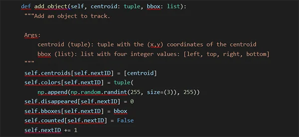
Conversely, we remove an object by deleting all data associated with the particular ObjectID:
Calculating distances and updating centroids
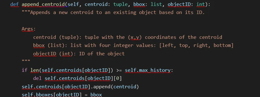
Note that we save a list of centroids instead of a single centroid. However, this list has a unique property: it has to have a length less than or equal to max_history. In that sense, we will only store the last max_history detected centroids, and we do that by deleting the first item of the list if its length is equal to the maximum and then appending the new centroid. Finally, we update the bounding box of the object with the last detection:
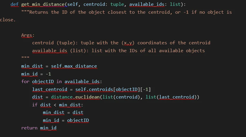
But how do we append the correct centroid to the object? As we said earlier, we use the Euclidean distance and append the centroid to the closest object, and we need a list of available IDs (as an object can only be updated once per frame) and the centroid to be appended. We calculate the Euclidean distance for each object and return the ID corresponding to the object closest to the new centroid. Note that if no object is close (when all distances are more significant than the maximum or no objects are available), this method returns -1:
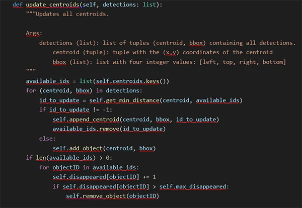
Finally, we use both helper methods in the primary centroid updater method. First, we set the available IDs as all current objects. Then, for each detection (defined by a tuple containing a bounding box and a centroid), we use the method get_min_distance to obtain the closest object. If the ID is valid, we append the detected centroid to the existing object and remove it from the available objects; if not, we create a new object. Finally, if there are no more detections but we still have available objects, we assume that these objects disappeared, removing the objects that disappeared max_disappeared times:
Updating and counting
There are two main methods in the Tracker class. The first is the update method, which uses a list of detections (defined the same way as before). If there are no detections, we assume that all objects disappeared, removing all objects that disappeared max_disappeared times. If there are no saved objects, we create objects for all detections. Finally, if there are saved objects and new detections, we update the centroids using the update_centroids method:
The second method is “count_people”, which iterates over all centroids that have not yet been counted. First, we calculate the direction the object is going towards with the difference between the mean of the previous centroids and the last centroid. If the object goes upwards, the last centroid is over the limit, and the mean of the previous centroids is under the limit. Then we count the object as entering the building. Similarly, if the object is going downwards, the last centroid is under the limit, and the mean of the previous centroids is over the limit, then the object is exiting the building:
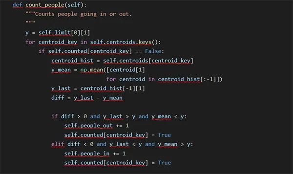
With the complete code, you can start identifying and tracking objects detected by any algorithm of your choice. For example, if you are processing a video frame by frame, you would get the bounding boxes and centroids of all objects and pass them to the update method of this class on each frame. Similarly, you can call the method count_people on every frame to update the counters based on the data that is stored at that moment.
Remember that, to use this object, you need to provide a bounding box and a centroid for all objects in each processed frame of a video. The following example was taken using an InceptionV2 implementation in the Jetson Inference library:
In this example, we use a video as input, detecting people in each frame and passing the corresponding bounding boxes and centroids to the Tracker object. Note that the quality of detections influences the tracking algorithm, so if your chosen detection algorithm fails to detect objects in a specific frame, the tracker could assume that the objects disappeared.
Conclusion
In this section, we explored a simple tracking algorithm and a counting algorithm that can be used together with any object detection algorithm or deep learning model. We defined the Tracker class, which uses bounding boxes and centroids to identify and keep track of moving objects in a video, using the Euclidean distance to associate new data with previous objects. Note that you have to tune the values for the number of times before an object disappears, the number of saved centroids, and the maximum distance between a centroid and new detections, to optimise the algorithm and get better performance.
EQUINOX
& COMPUTER VISION
Discover how we apply Computer Vision to comprehensive solutions for different industries and business challenges
